Hi Pythonistas!
Let start another post in AI journey: let's break down derivatives and gradient descent on the simple function
f(x)=x^2.I'll keep it super clear, easy, and show you where this magic is used in the real world.
What's a Derivative?
A derivative tells you how 'steep' a function is and which way it’s going like if you’re walking on a hill,
is it going up or down, and how quickly?
For our hill:
f(x)=x^2
The derivative is:
f′(x)=2x
So if you’re at x=3, the slope is 2×3=6 (pretty steep uphill).
If you’re at x=0x=0, the slope is 0 (flat ground bottom of the hill!).
What Is Gradient Descent?
Gradient descent is how computers 'find the bottom of the hill' on any curve:
- You start somewhere (random x)
- Feel the slope: If it's positive, go left. If it's negative, go right.
- Take a small step downhill (not up!).
- Repeat until you can't go lower (the bottom!)
This is how a computer 'learns' how to improve by following the steepest path downward to the lowest point.
What is significance of the lowest point
Lowest point on the graph is point where the error is minimal. By using gradient find the lowest point so that the
model can predict the result as accurate as possible
Python Demo (Walk Down the Hill!)
import numpy as np
import matplotlib.pyplot as plt

def f(x):
    return x**2

def df(x):
    return 2*x

def gradient_descent(start_x, learning_rate, max_steps, tolerance=1e-6):
    x = start_x
    history = [x]
    for _ in range(max_steps):
        grad = df(x)
        if abs(grad) < tolerance:
            print(f"Stopped early: slope is nearly flat at x = {x}")
            break
        x -= learning_rate * grad
        history.append(x)
    return history

# Parameters
start_x = 8
learning_rate = 0.1
max_steps = 50

path = gradient_descent(start_x, learning_rate, max_steps)

# Visualization
x_vals = np.linspace(-9, 9, 200)
plt.plot(x_vals, f(x_vals), label='f(x) = x^2')
plt.scatter(path, [f(x) for x in path], color='red', zorder=5, label='Gradient Descent Steps')
plt.plot(path, [f(x) for x in path], '--r')
plt.title('Walking Down the Hill (Gradient Descent)')
plt.xlabel('x')
plt.ylabel('f(x)')
plt.legend()
plt.grid()
plt.show()
Output
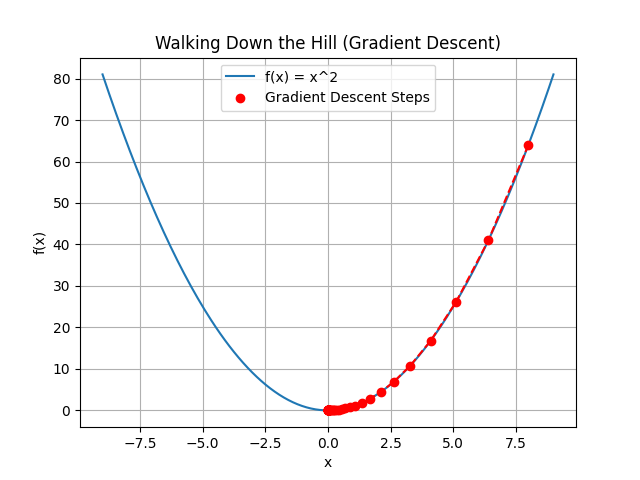
Run this and you'll see "steps" in red, starting at x=8x=8 and marching toward x=0x=0, which is the lowest point.
Where Is This Used in Real Life?
- Training AI/ML Models: Every time you 'fit' a model, it’s using gradient descent to find the best answer like finding the very bottom of a hill, but in many dimensions at once.
- Predicting Stocks/Prices: Algorithms use gradient descent to tune themselves for best predictions.
- Robotics: Robots tune movements using this math, learning smooth actions.
- Business Decisions: Companies minimize costs (the "bottom of the hill") with gradient descent-style math.
What I Learned
- Derivative: Tells you the steepness and direction.
- Gradient Descent: Step-by-step path, always moving downhill to reach the lowest point.
Try playing with the starting point, the learning rate, or function see how it changes your path!
What’s Next
In the upcoming post we learn about the basics of docker